Since the latest release of TMS Cloud Pack, there is now also built-in support to use Google Firebase for cloud data storage. The architecture of Google's Firebase is quite simple. It offers storage of JSON data in the cloud. The JSON data has a unique identifier in a table and via access with this unique identifier, this JSON data can be read, updated or deleted. In addition, indexing rules can be set to perform query on the data in a Firebase table, for example, retrieve all JSON objects where a field X has value Y.
To make it really easy use to use data on Google Firebase from a Delphi or C++Builder application, we have added capabilities to put objects or generic lists of objects in a Firebase table. This is done via the non-visual component TFirebaseObjectDatabase that you can put on the form.
![]()
To demonstrate this, consider a class we want to use in the Delphi application that descends from TFirebaseObject:
  TFirebaseCustomer = class(TFirebaseObject)
  private
    FName: string;
    FStreet: string;
    FZIP: integer;
    FDoB: TDate;
    FCity: string;
  public
    constructor Create; override;
    destructor Destroy; override;
  published
    property Name: string read FName write FName;
    property Street: string read FStreet write FStreet;
    property City: string read FCity write FCity;
    property ZIP: integer read FZIP write FZIP;
    property DoB: TDate read FDoB write FDoB;
  end;
Now, after we have retrieved a connection for TAdvFirebaseObjectDataBase to Firebase via:
  AdvFirebaseObjectDatabase1.DatabaseName := 'TMS';
  AdvFirebaseObjectDatabase1.TableName := 'Customers';
  AdvFirebaseObjectDatabase1.Connect;
we can create and put TFirebaseCustomer objects in the Google Firebase realtime data cloud:
var
  cst: TFireBaseCustomer;
begin
  cst := TFireBaseCustomer.Create;
  try
    cst.Name := 'Bill Gates';
    cst.Street := 'Microsoft Av';
    cst.ZIP := 2123;
    cst.City := 'Redmond';
    cst.DoB := EncodeDate(1969,04,18);
    cst.ID := '1240';
    AdvFirebaseObjectDatabase1.InsertObject(cst);
  finally
    cst.Free;
  end;
end;
All published properties of the object will be automatically persisted on the Google Firebase cloud. This is how the data looks when inspecting it on the
Firebase console
![]()
Note that we have explicitly set the unique ID of the object via the cst.ID property. When the ID is set at application level, it is the responsibility of the app to use unique IDs. When no ID is set, the AdvFirebaseObjectDatabase will automatically create a GUID as ID.
In this example, we have created a rather simple object with simple data types. But nothing prevents you from using class properties as in this example:
  TCareerPeriod = class(TPersistent)
  private
    FFinish: integer;
    FStart: integer;
  published
    property Start: integer read FStart write FStart;
    property Finish: integer read FFinish write FFinish;
  end;

  TFirebaseCustomer = class(TFirebaseObject)
  private
    FName: string;
    FStreet: string;
    FZIP: integer;
    FDoB: TDate;
    FCity: string;
    FPicture: TFireBasePicture;
    FCareer: TCareerPeriod;
    procedure SetCareer(const Value: TCareerPeriod);
  public
    constructor Create; override;
    destructor Destroy; override;
  published
    property Name: string read FName write FName;
    property Street: string read FStreet write FStreet;
    property City: string read FCity write FCity;
    property ZIP: integer read FZIP write FZIP;
    property DoB: TDate read FDoB write FDoB;
    property Career: TCareerPeriod read FCareer write SetCareer;
  end;
And now this code can be used to persist this slightly more complex object:
var
  cst: TFireBaseCustomer;
begin
  cst := TFireBaseCustomer.Create;
  try
    cst.Name := 'Elon Musk';
    cst.Street := '3500 Deer Creek Road';
    cst.ZIP := 2123;
    cst.City := 'Palo Alto';
    cst.DoB := EncodeDate(1975,03,21);
    cst.ID := '1241';
    cst.Career.Start := 2011;
    cst.Career.Finish := 2017;
    AdvFirebaseObjectDatabase1.InsertObject(cst);
  finally
    cst.Free;
  end;
end;
As you can see, more complex classes can be easily & automatically persisted in the Google Firebase cloud.
![]()
With respect to types of fields, there is one caveat though, Google Firebase doesn't offer out of the box support for binary blobs. Imagine that we'd want to persist a Delphi object that has a TPicture property. The TPicture is internally streamed in a custom way to the DFM (via the DefineProperties(Filer: TFiler); override) and the JSON persister does not automatically get this data. There is however an easy workaround to add a published string property to a class descending from TPicture and use this string to hold hex encoded binary data of the picture. The DataString property getter & setter methods use the StreamToHex() and HexToStream() functions that are included in the unit CloudCustomObjectFirebase:
  TFireBasePicture = class(TPicture)
  private
    function GetDataString: string;
    procedure SetDataString(const Value: string);
  published
    property DataString: string read GetDataString write SetDataString;
  end;


{ TFireBasePicture }

function TFireBasePicture.GetDataString: string;
var
  ms: TMemoryStream;
begin
  ms := TMemoryStream.Create;
  try
    SaveToStream(ms);
    Result := StreamToHex(ms);
  finally
    ms.Free;
  end;
end;

procedure TFireBasePicture.SetDataString(const Value: string);
var
  ms: TMemoryStream;
begin
  ms := HexToStream(Value);
  try
    LoadFromStream(ms);
  finally
    ms.Free;
  end;
end;
This way, we can extend the class to have a picture property:
  TFireBaseCustomer = class(TFirebaseObject)
  private
    FName: string;
    FStreet: string;
    FZIP: integer;
    FDoB: TDate;
    FCity: string;
    FPicture: TFireBasePicture;
    FCareer: TCareerPeriod;
    procedure SetPicture(const Value: TFireBasePicture);
    procedure SetCareer(const Value: TCareerPeriod);
  public
    constructor Create; override;
    destructor Destroy; override;
  published
    property Name: string read FName write FName;
    property Street: string read FStreet write FStreet;
    property City: string read FCity write FCity;
    property ZIP: integer read FZIP write FZIP;
    property DoB: TDate read FDoB write FDoB;
    property Career: TCareerPeriod read FCareer write SetCareer;
    property Picture: TFireBasePicture read FPicture write SetPicture;
  end;
and persist the object with picture via:
var
  cst: TFireBaseCustomer;
begin
  cst := TFireBaseCustomer.Create;
  try
    cst.Name := 'Tim Cook';
    cst.Street := '1 Infinite Loop';
    cst.ZIP := 2123;
    cst.City := 'Cupertino';
    cst.DoB := EncodeDate(1975,03,21);
    cst.ID := '1242';
    cst.Picture.LoadFromFile('tim_cook.jpg');
    cst.Career.Start := 2006;
    cst.Career.Finish := 2017;

    AdvFirebaseObjectDatabase1.InsertObject(cst);
  finally
    cst.Free;
  end;
end;
To retrieve the objects back that were persisted, we can use:
var
  fbo: TFirebaseObject;
begin
  fbo := AdvFirebaseObjectDatabase1.ReadObject('1240');

  if Assigned(fbo) then
  begin
    if (fbo is TFirebaseCustomer) then
      ShowMessage((fbo as TFirebaseCustomer).Name+';'+(fbo as TFirebaseCustomer).City);
    fbo.Free;
  end;
end;
To persist a property change of the object, for example to change the career date of customer 1241 to 2018, we could write:
var
  fbo: TFirebaseObject;
begin
  fbo := AdvFirebaseObjectDatabase1.ReadObject('1241');

  if Assigned(fbo) then
  begin
    if (fbo is TFirebaseCustomer) then
    begin
      ((fbo as TFirebaseCustomer).Career.Finish := 2018;
      AdvFirebaseObjectDatabase1.WriteObject(fbo);
    end;
  end;
end;
Working with generic lists
The previous samples all showed how to perform CRUD operations on single objects in the Google Firebase cloud. Our component TAdvFirebaseObjectDatabase also facilitates dealing with generic lists of objects. Imagine you want to persist a score table of game and have following simple classes to store this:
  TSimpleClass = class(TFirebaseObject)
  private
    FName: string;
    FScore: integer;
  published
    property Name: string read FName write FName;
    property Score: integer read FScore write FScore;
  end;

  TSimpleList = TList<TSimpleClass>;
With this class and its generic list, we can add a list of data at once in the Google Firebase cloud:
var
  sl: TFirebaseObjectList;
  sc: TSimpleClass;
  I: Integer;
begin
  sl := TFirebaseObjectList.Create;
  try
    sc := TSimpleClass.Create;
    sc.Name := 'Bruno';
    sc.Score := 48;
    sc.ID := '1';
    sl.Add(sc);

    sc := TSimpleClass.Create;
    sc.Name := 'Nancy';
    sc.Score := 83;
    sc.ID := '2';
    sl.Add(sc);

    sc := TSimpleClass.Create;
    sc.Name := 'Pieter';
    sc.Score := 17;
    sc.ID := '3';
    sl.Add(sc);

    sc := TSimpleClass.Create;
    sc.Name := 'Bart';
    sc.Score := 299;
    sc.ID := '4';
    sl.Add(sc);

    sc := TSimpleClass.Create;
    sc.Name := 'Wagner';
    sc.Score := 55;
    sc.ID := '5';
    sl.Add(sc);

    AdvFirebaseObjectDatabase1.TableName:= 'List';
    AdvFirebaseObjectDatabase1.InsertList(sl);

    for I := 0 to sl.Count - 1 do
      sl[I].Free;
  finally
    sl.Free;
  end;
end;
Inspecting this on the Google Firebase console results in:
![]()
If at a later time we'd like to retrieve the score of Bart, we could use the code:
var
  c: TFirebaseObjectList;
  I: Integer;

begin
  AdvFirebaseObjectDatabase1.TableName := 'List';
  c:= AdvFirebaseObjectDatabase1.QueryList('Name', 'Bart');
  if Assigned(c) then
  begin
    for I := 0 to c.Count - 1 do
    begin
      ShowMessage((c[I] as TSimpleClass).Score.ToString);
      c[I].Free;
    end;
    c.Free;
  end;
end;
This performs a query on the List table for value 'Bart' set in the 'Name' field. The result of the query is a generic list (in case multiple matching results are found).
This was a glimpse at the TAdvFirebaseObjectDataBase component as an introduction for the new Google Firebase access features in the
TMS Cloud Pack. Explore the full set of powerful capabilities of TAdvFirebaseObjectDataBase and the many other components in
TMS Cloud Pack to make consuming cloud services in Delphi & C++Builder a piece of cake.


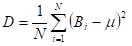 where µ is the mean value
  N is the number of elements.
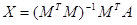 where MT is the transposed matrix, 1 means the inversed matrix.


